Getting Started with Machine Learning using Python

So you've decided to dive into machine learning with Python? Good choice! I remember when I first started – it felt like trying to drink from a fire hose. There's so much information out there, and half the tutorials assume you already know what you're doing. Don't worry though, I've been there, made all the mistakes, and I'm going to walk you through this step by step.

Machine learning isn't as scary as it sounds. Yeah, there's math involved, but you don't need a PhD to get started. What you do need is curiosity, patience, and a willingness to break things (trust me, you'll break a lot of code at first, and that's totally normal).

Why Python for Machine Learning? Because Life's Too Short for Complex Syntax

Before we jump into the code, let's talk about why Python has become the go-to language for ML. It's not because data scientists are lazy (well, maybe a little), but because Python just makes sense. The syntax is clean, there are incredible libraries that do the heavy lifting for you, and the community is massive – which means when you get stuck at 2 AM debugging your model, someone on Stack Overflow has probably already solved your problem.

Python's readable syntax makes machine learning accessible to everyone

The real magic happens when you combine Python with libraries like scikit-learn, pandas, and numpy. These aren't just tools – they're like having a team of data science experts built into your code. You can implement complex algorithms with just a few lines of code, which means you spend more time understanding your data and less time wrestling with implementation details.

Setting Up Your Machine Learning Environment (The Right Way)

Alright, let's get our hands dirty. First things first – you need to set up your environment properly. I've seen too many people skip this step and then wonder why their code doesn't work or why they're constantly dealing with version conflicts.

Here's what you need to install. I'm assuming you already have Python 3.7+ installed (if not, go grab it from python.org). We're going to use pip to install our packages, but I highly recommend using a virtual environment to keep things clean:

# Create a virtual environment
python -m venv ml_env

# Activate it (on Windows)
ml_env\Scripts\activate

# Activate it (on Mac/Linux)
source ml_env/bin/activate

# Install the essential packages
pip install numpy pandas matplotlib seaborn scikit-learn jupyter

Now, let me tell you about each of these packages because understanding what they do will save you hours of confusion later:

• NumPy – This is your mathematical foundation. It handles arrays and matrices efficiently, which is basically everything in ML
• Pandas – Your data manipulation swiss army knife. If you're working with CSV files, databases, or any structured data, pandas is your best friend
• Matplotlib & Seaborn – For creating visualizations. Trust me, you'll need to plot your data more than you think
• Scikit-learn – The star of the show. This library contains most of the ML algorithms you'll ever need
• Jupyter – Interactive notebooks that make experimentation so much easier

Your First Machine Learning Program (It's Simpler Than You Think)

Let's start with something simple but real – predicting house prices. I know, I know, every ML tutorial uses this example, but there's a good reason for it. It's intuitive, the relationship between features and target is clear, and you can actually understand what's happening.

Here's our first complete machine learning program:

import pandas as pd
import numpy as np
from sklearn.model_selection import train_test_split
from sklearn.linear_model import LinearRegression
from sklearn.metrics import mean_squared_error, r2_score
import matplotlib.pyplot as plt

# Create some sample data (in real life, you'd load this from a file)
np.random.seed(42)  # for reproducible results
n_samples = 1000

# Generate synthetic house data
square_feet = np.random.normal(2000, 500, n_samples)
bedrooms = np.random.poisson(3, n_samples)
age = np.random.uniform(0, 50, n_samples)

# Create a realistic price relationship
price = (square_feet * 100 + bedrooms * 5000 - age * 1000 + 
         np.random.normal(0, 10000, n_samples))

# Put it in a DataFrame (pandas loves DataFrames)
data = pd.DataFrame({
    'square_feet': square_feet,
    'bedrooms': bedrooms,
    'age': age,
    'price': price
})

print("First 5 rows of our data:")
print(data.head())
print(f"\nDataset shape: {data.shape}")

This creates a synthetic dataset, but it mimics real-world data pretty well. We have houses with different square footage, number of bedrooms, and ages, and we're trying to predict the price.

Data visualization is crucial for understanding your dataset

Understanding algorithms helps you choose the right tool

Now let's actually build and train our model:

# Separate features (X) and target (y)
X = data[['square_feet', 'bedrooms', 'age']]
y = data['price']

# Split data into training and testing sets
X_train, X_test, y_train, y_test = train_test_split(
    X, y, test_size=0.2, random_state=42
)

# Create and train the model
model = LinearRegression()
model.fit(X_train, y_train)

# Make predictions
y_pred = model.predict(X_test)

# Evaluate the model
mse = mean_squared_error(y_test, y_pred)
r2 = r2_score(y_test, y_pred)

print(f"Mean Squared Error: {mse:.2f}")
print(f"R² Score: {r2:.2f}")
print(f"Root Mean Squared Error: {np.sqrt(mse):.2f}")

# Let's see what the model learned
print("\nModel coefficients:")
for feature, coef in zip(X.columns, model.coef_):
    print(f"{feature}: {coef:.2f}")
print(f"Intercept: {model.intercept_:.2f}")

What's happening here? We're splitting our data into training and testing sets (this is crucial – never test on data you trained on!), creating a linear regression model, training it on our training data, and then evaluating how well it performs on unseen test data.

The biggest mistake beginners make is not splitting their data properly. Your model might seem amazing, but if you're testing on the same data you trained on, you're basically asking it to remember the answers to a test it already took.

Hard-learned lesson from my early ML days

Understanding What Your Model Actually Learned

Let's visualize our results to see how well our model is doing. This is where the magic of matplotlib comes in:

# Create a scatter plot of actual vs predicted prices
plt.figure(figsize=(10, 6))
plt.scatter(y_test, y_pred, alpha=0.6)
plt.plot([y_test.min(), y_test.max()], [y_test.min(), y_test.max()], 'r--', lw=2)
plt.xlabel('Actual Price')
plt.ylabel('Predicted Price')
plt.title('Actual vs Predicted House Prices')
plt.show()

# Let's make a prediction on a new house
new_house = pd.DataFrame({
    'square_feet': [2500],
    'bedrooms': [4],
    'age': [10]
})

predicted_price = model.predict(new_house)
print(f"\nPredicted price for a 2500 sq ft, 4-bedroom, 10-year-old house: ${predicted_price[0]:,.2f}")

This visualization is super important. If your points are scattered all over the place, your model isn't learning the relationship between features and target very well. If they're close to the diagonal line, you're in good shape.

Diving Deeper: Classification Problems

Alright, predicting continuous values like house prices is cool, but what about classification – predicting categories? Let's tackle a classic problem: determining if an email is spam or not. This is where things get interesting because we're dealing with text data.

from sklearn.feature_extraction.text import TfidfVectorizer
from sklearn.naive_bayes import MultinomialNB
from sklearn.pipeline import Pipeline
from sklearn.metrics import classification_report, confusion_matrix

# Sample email data (in practice, you'd have thousands of these)
emails = [
    "Get rich quick! Click here now!",
    "Meeting scheduled for tomorrow at 3pm",
    "FREE MONEY!!! Act now!!!",
    "Please review the attached document",
    "You've won a million dollars! Claim now!",
    "Can we reschedule our call?",
    "URGENT: Your account will be closed!",
    "Thanks for the great presentation today",
    "Buy now and save 90%!!!",
    "Looking forward to our discussion"
]

# Labels (0 = not spam, 1 = spam)
labels = [1, 0, 1, 0, 1, 0, 1, 0, 1, 0]

# Create a pipeline that combines text processing and classification
pipeline = Pipeline([
    ('tfidf', TfidfVectorizer(stop_words='english')),
    ('classifier', MultinomialNB())
])

# Train the model
pipeline.fit(emails, labels)

# Test on new emails
test_emails = [
    "Important meeting tomorrow",
    "WIN BIG MONEY NOW!!!",
    "Project deadline reminder"
]

predictions = pipeline.predict(test_emails)
probabilities = pipeline.predict_proba(test_emails)

for email, pred, prob in zip(test_emails, predictions, probabilities):
    status = "SPAM" if pred == 1 else "NOT SPAM"
    confidence = max(prob) * 100
    print(f"'{email}' -> {status} (confidence: {confidence:.1f}%)")

This example introduces some important concepts. We're using a Pipeline (which chains preprocessing and modeling steps together), TF-IDF vectorization (which converts text into numbers), and Naive Bayes (a probabilistic classifier that works great with text).

Real-World Data Is Messy (And That's Okay)

Let me tell you something – the examples above are clean and perfect, but real data is never like that. It's messy, has missing values, contains outliers, and generally tries to make your life difficult. Let's look at how to handle this:

import pandas as pd
import numpy as np
from sklearn.impute import SimpleImputer
from sklearn.preprocessing import StandardScaler, LabelEncoder
from sklearn.ensemble import RandomForestClassifier

# Create some messy data (this is more realistic)
messy_data = pd.DataFrame({
    'age': [25, 35, np.nan, 45, 30, np.nan, 50],
    'income': [50000, 80000, 60000, np.nan, 70000, 55000, 90000],
    'education': ['Bachelor', 'Master', 'PhD', 'Bachelor', 'Master', 'High School', 'PhD'],
    'purchased': [0, 1, 1, 1, 0, 0, 1]
})

print("Original messy data:")
print(messy_data)
print(f"\nMissing values:\n{messy_data.isnull().sum()}")

# Handle missing values
# For numerical columns, use median
num_imputer = SimpleImputer(strategy='median')
messy_data['age'] = num_imputer.fit_transform(messy_data[['age']])
messy_data['income'] = num_imputer.fit_transform(messy_data[['income']])

# For categorical columns, encode them as numbers
le = LabelEncoder()
messy_data['education_encoded'] = le.fit_transform(messy_data['education'])

print("\nCleaned data:")
print(messy_data)

# Now we can train a model
X = messy_data[['age', 'income', 'education_encoded']]
y = messy_data['purchased']

# Scale the features (important for many algorithms)
scaler = StandardScaler()
X_scaled = scaler.fit_transform(X)

# Use Random Forest (handles various data types well)
rf = RandomForestClassifier(n_estimators=100, random_state=42)
rf.fit(X_scaled, y)

# Feature importance (what factors matter most?)
feature_names = ['age', 'income', 'education_encoded']
importance = rf.feature_importances_

print("\nFeature importance:")
for name, imp in zip(feature_names, importance):
    print(f"{name}: {imp:.3f}")

This shows you the dirty work that goes into real ML projects. Data cleaning and preprocessing often takes 80% of your time, and the actual modeling is just 20%. Don't get discouraged by this – it's normal!

Model Evaluation: Because "It Works" Isn't Good Enough

Here's where a lot of beginners mess up. They build a model, see that it gives predictions, and assume it's working well. But how do you know if your model is actually good? You need proper evaluation metrics.

from sklearn.model_selection import cross_val_score, GridSearchCV
from sklearn.metrics import accuracy_score, precision_score, recall_score, f1_score

# Let's create a more comprehensive evaluation
def evaluate_model(model, X, y):
    """
    Comprehensive model evaluation function
    """
    # Cross-validation gives us a better estimate of model performance
    cv_scores = cross_val_score(model, X, y, cv=5, scoring='accuracy')
    
    print(f"Cross-validation accuracy: {cv_scores.mean():.3f} (+/- {cv_scores.std() * 2:.3f})")
    
    # Fit the model and get detailed metrics
    X_train, X_test, y_train, y_test = train_test_split(X, y, test_size=0.3, random_state=42)
    model.fit(X_train, y_train)
    y_pred = model.predict(X_test)
    
    print(f"Test accuracy: {accuracy_score(y_test, y_pred):.3f}")
    print(f"Precision: {precision_score(y_test, y_pred, average='weighted'):.3f}")
    print(f"Recall: {recall_score(y_test, y_pred, average='weighted'):.3f}")
    print(f"F1-score: {f1_score(y_test, y_pred, average='weighted'):.3f}")
    
    return model

# Load a real dataset for demonstration
from sklearn.datasets import load_wine
wine_data = load_wine()
X, y = wine_data.data, wine_data.target

# Compare different algorithms
models = {
    'Random Forest': RandomForestClassifier(random_state=42),
    'Naive Bayes': MultinomialNB(),
    'Linear Regression': LinearRegression()
}

print("Model comparison on wine dataset:")
for name, model in models.items():
    print(f"\n{name}:")
    try:
        evaluate_model(model, X, y)
    except Exception as e:
        print(f"Error with {name}: {e}")

Don't fall in love with your first model. Try different algorithms, compare their performance, and always validate your results. The best data scientists are skeptics of their own work.

Advice that saved me from many embarrassing mistakes

Hyperparameter Tuning: Making Your Models Actually Good

Once you've got a basic model working, you'll want to tune it. Think of hyperparameters as the settings on your model – like adjusting the temperature on your oven. The wrong settings can ruin your results, but the right ones can make them amazing.

from sklearn.model_selection import GridSearchCV
from sklearn.ensemble import RandomForestClassifier

# Define the parameter grid to search
param_grid = {
    'n_estimators': [50, 100, 200],
    'max_depth': [None, 10, 20, 30],
    'min_samples_split': [2, 5, 10],
    'min_samples_leaf': [1, 2, 4]
}

# Create the model
rf = RandomForestClassifier(random_state=42)

# Use GridSearchCV to find the best parameters
grid_search = GridSearchCV(
    estimator=rf,
    param_grid=param_grid,
    cv=5,
    scoring='accuracy',
    n_jobs=-1,  # Use all available cores
    verbose=1   # Show progress
)

print("Searching for best parameters...")
grid_search.fit(X, y)

print(f"Best parameters: {grid_search.best_params_}")
print(f"Best cross-validation score: {grid_search.best_score_:.3f}")

# Use the best model
best_model = grid_search.best_estimator_

This might take a while to run (hence the verbose=1 to show progress), but it's worth it. GridSearchCV tries every combination of parameters you specify and tells you which works best.

Common Pitfalls and How to Avoid Them

Let me share some mistakes I've made (and seen others make) so you can avoid them:

• Data leakage – This is when information from your target variable somehow gets into your features. It makes your model look amazing but perform terribly in real life
• Overfitting – Your model memorizes the training data instead of learning general patterns. Use cross-validation and keep your models simple at first
• Not understanding your data – Always explore your data first. Plot histograms, check for correlations, look for outliers
• Ignoring feature scaling – Some algorithms (like neural networks and SVM) are very sensitive to the scale of your features. Normalize or standardize when needed
• Using accuracy for imbalanced datasets – If you have 95% of one class and 5% of another, a dumb model that always predicts the majority class will have 95% accuracy but be completely useless

What's Next? Your Machine Learning Journey

Congratulations! If you've made it this far and actually ran the code examples, you're no longer a complete beginner. You understand the basic workflow of machine learning, you've seen how to handle messy data, and you know how to evaluate your models properly.

But this is just the beginning. Here's what I'd recommend for your next steps:

• Practice with real datasets from Kaggle or UCI ML Repository
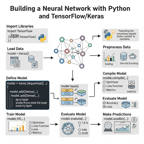
• Learn about deep learning with TensorFlow or PyTorch (but master the basics first!)
• Understand different problem types: time series, computer vision, natural language processing
• Learn about feature engineering – often more important than fancy algorithms
• Get comfortable with SQL and data visualization tools

The most important advice I can give you is this: start building projects. Don't just follow tutorials (though they're great for learning concepts). Find a problem you're genuinely interested in solving and try to solve it with machine learning. You'll learn more from one real project than from ten tutorials.

Machine learning is a journey, not a destination. The field evolves rapidly, new techniques emerge constantly, and there's always something new to learn. But that's what makes it exciting! You're joining a community of people who are literally reshaping how we interact with technology and solve problems.

Remember, every expert was once a beginner. The key is to keep experimenting, keep learning, and don't be afraid to make mistakes. Some of my best insights came from bugs in my code that led me down unexpected paths. Happy coding, and welcome to the world of machine learning!